Example single fit
Fitting method
Read data
Select and create model
Fit the data with model
Save plots and log
Quick fit
import src.binary_sed_fitting as bsf
################################################################################
name        = 'WOCS2002'
file_name   = 'data/extinction_corrected_flux_files/%s.csv'%name
data        = bsf.load_data(file_name, mode='csv')
distance    = 831. # pc
e_distance  = 11.  # pc
################################################################################
model_name = 'kurucz'
limits = {'Te'   : [3500, 9000],
          'logg' : [   3,    5],
          'MH'   : [ 0.0,  0.0],
          'alpha': [ 0.0,  0.0]}
model = bsf.Model(model_name, limits=limits)
################################################################################
star = bsf.Star(name=name,
                distance=distance,
                e_distance=e_distance,
                data=data,
                model=model)
################################################################################
star.fit_chi2()
star.plot()
22:39:52 ----- WARNING  ----- estimate_runtime
Calculating chi2: ETA ~ 0 s
Selecting model
Supported models: Kurucz, Koester and Kurucz_UVBLUE
import src.binary_sed_fitting as bsf
################################################################################
model_name = 'kurucz'
limits = {'Te'   : [3500, 9000],
          'logg' : [   3,    5],
          'MH'   : [ 0.0,  0.0],
          'alpha': [ 0.0,  0.0]}
model = bsf.Model(model_name, limits=limits)
print(model_name, '\n\n\n' ,model.da)
################################################################################
model_name = 'kurucz_uvblue'
limits = {'Te'   : [3500, 9000],
          'logg' : [   3,    5],
          'MH'   : [ 0.0,  0.0]}
model = bsf.Model(model_name, limits=limits)
print(model_name, '\n\n\n' ,model.da)
################################################################################
model_name = 'koester'
limits = {'Te'   : [5000, 80000],
          'logg' : [ 6.5,   9.5]}
model = bsf.Model(model_name, limits=limits)
print(model_name, '\n\n\n' ,model.da)
kurucz


 <xarray.DataArray (FilterID: 8162, Te: 23, logg: 5, MH: 1, alpha: 1)> Size: 8MB
[938630 values with dtype=float64]
Coordinates:
  * FilterID  (FilterID) <U38 1MB 'Swift/UVOT.UVM2_fil' ... 'QUIJOTE/MFI.11GH...
  * Te        (Te) int32 92B 3500 3750 4000 4250 4500 ... 8250 8500 8750 9000
  * logg      (logg) float64 40B 3.0 3.5 4.0 4.5 5.0
  * MH        (MH) float64 8B 0.0
  * alpha     (alpha) float64 8B 0.0
Attributes:
    Wavelengths:  [1.19128077e+00 1.24254209e+00 1.48134125e+02 ... 3.8683349...
    unit:         erg/s/cm2/A
    long_name:    Flux
kurucz_uvblue


 <xarray.DataArray (FilterID: 8162, Te: 12, logg: 5, MH: 1)> Size: 4MB
[489720 values with dtype=float64]
Coordinates:
  * FilterID  (FilterID) <U38 1MB 'Swift/UVOT.UVM2_fil' ... 'QUIJOTE/MFI.11GH...
  * Te        (Te) int32 48B 3500 4000 4500 5000 5500 ... 7500 8000 8500 9000
  * logg      (logg) float64 40B 3.0 3.5 4.0 4.5 5.0
  * MH        (MH) float64 8B 0.0
    alpha     float64 8B ...
Attributes:
    Wavelengths:  [1.19128077e+00 1.24254209e+00 1.48134125e+02 ... 3.8683349...
    unit:         erg/s/cm2/A
    long_name:    Flux
koester


 <xarray.DataArray (FilterID: 8162, Te: 82, logg: 13)> Size: 70MB
[8700692 values with dtype=float64]
Coordinates:
  * FilterID  (FilterID) <U38 1MB 'IUE/IUE.1250-1300' ... 'QUIJOTE/MFI.11GHz_H3'
  * Te        (Te) int32 328B 5000 5250 5500 5750 ... 50000 60000 70000 80000
  * logg      (logg) float64 104B 6.5 6.75 7.0 7.25 7.5 ... 8.75 9.0 9.25 9.5
Attributes:
    Wavelengths:  [1.28470318e+03 1.35336435e+03 1.35623969e+03 ... 3.8683349...
    unit:         erg/s/cm2/A
    long_name:    Flux
Recommended fitting routine
Starname: Name of the stardistance,e_distance: Distance and it’s error in pcfilters_to_drop: Filters to be removed from the fit (due to bad data, bad fit, saturation…)wavelength_range: Wavelength range to be fitted in Angstromdata: DataFrame with the photometric fluxmodel: Model object of required model and parameter limitsr_limits: 2 optionsblackbody: Radius range automatically calculated from blackbody fit[r_min,r_max]: Radius is varied between the r_min and r_max given in solar radii
run_name: A string name for tracking different fits
fit_chi2Calculates chi2 for the data and model.
refitif
True: the fit is redone.If
False: If a previous fit is available, it is read. Otherwise a fresh fit is made.
fit_noisy_chi2Fits chi2 by adding noise to the data. Useful for getting statistical errors.
refit: ifTruethe fit is redone. IfFalse, the previous fit is read.
plotadd_noisy_seds: Whether to plot the noisy SEDs.folder: Folder for saving the plotFR_cutoff: Fractional residual cutoff for indicating excess flux
plot_publicPlots a smaller plot with SED, FR and EWR
save_summarySaves the fit parameters in a logfile
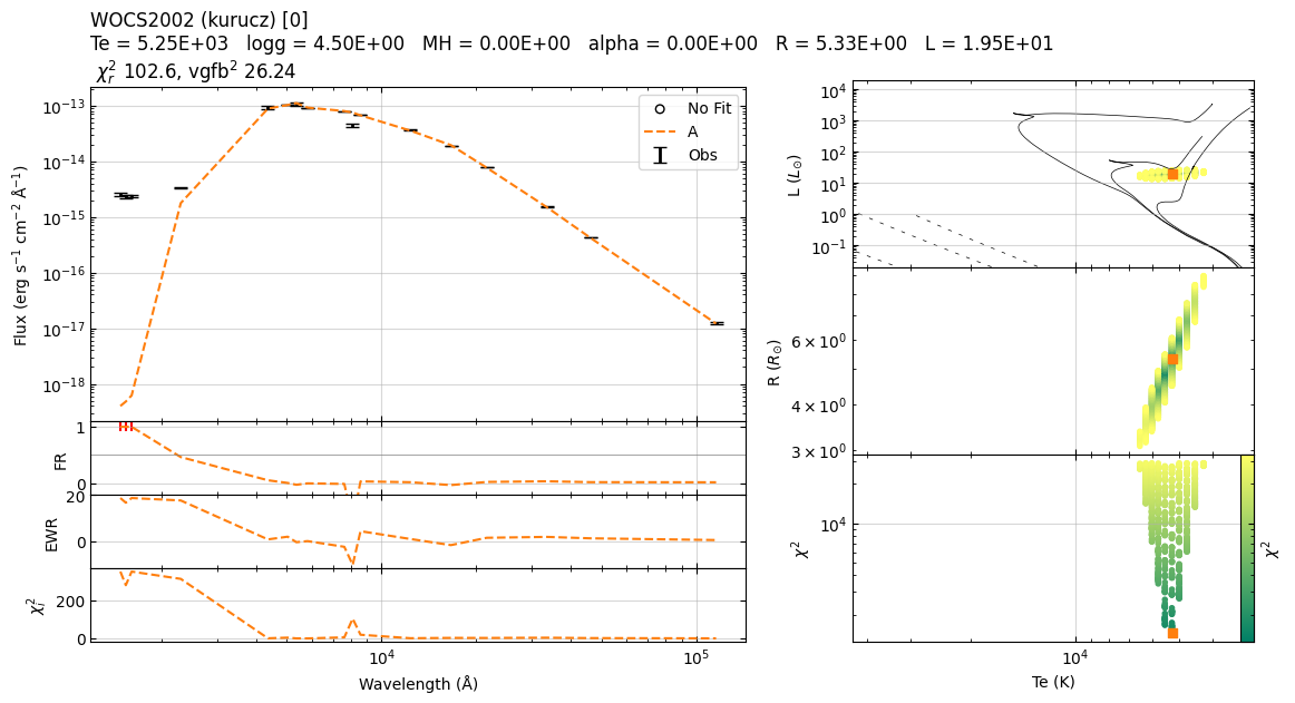
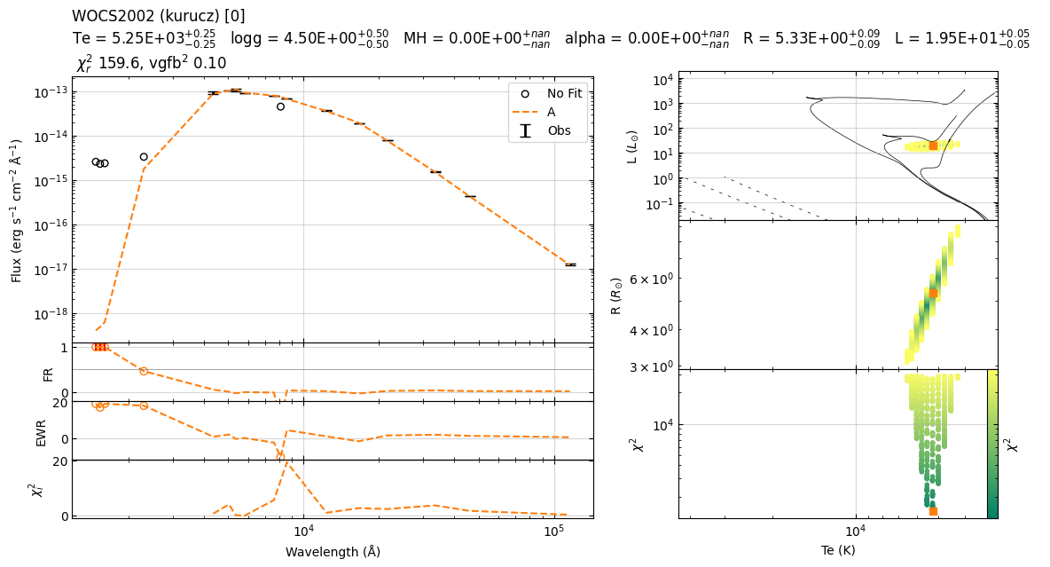
Example 1
import src.binary_sed_fitting as bsf
import warnings
warnings.filterwarnings("ignore")
bsf.console.setLevel(bsf.logging.INFO)
################################################################################
name = 'WOCS2002'
file_name = 'data/extinction_corrected_flux_files/%s.csv'%name
data = bsf.load_data(file_name, mode='csv')
distance = 831. # pc
e_distance = 11. # pc
refit = False
run_name = '0'
################################################################################
model_name = 'kurucz'
limits = {'Te' : [3500, 9000],
'logg' : [ 3, 5],
'MH' : [ 0.0, 0.0],
'alpha': [ 0.0, 0.0]}
model = bsf.Model(model_name, limits=limits)
################################################################################
star = bsf.Star(name=name,
distance=distance,
e_distance=e_distance,
filters_to_drop=['KPNO/Mosaic.I'],
wavelength_range=[3000, 1_000_000_000],
data=data,
model=model,
r_limits='blackbody',
run_name=run_name)
################################################################################
star.fit_chi2(refit=refit)
star.fit_noisy_chi2(refit=refit)
################################################################################
star.plot(add_noisy_seds=False,
folder='plots/',
FR_cutoff=0.5)
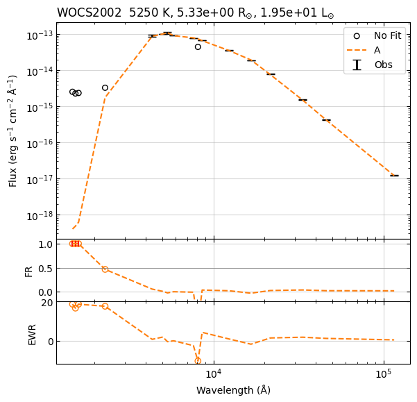
star.plot_public(add_noisy_seds=False,
folder='plots/',
FR_cutoff=0.5)
################################################################################
star.save_summary()
22:39:54 ----- INFO     ----- __init__
==========================================================
----------------------------------------------------------
------------            WOCS2002 A            ------------
----------------------------------------------------------
==========================================================
22:39:54 ----- INFO     ----- drop_filters
                        Fitted           Not fitted
wavelength
1481.000000                     Astrosat/UVIT.F148W
1541.000000                     Astrosat/UVIT.F154W
1608.000000                     Astrosat/UVIT.F169M
2303.366368                         GALEX/GALEX.NUV
4357.276538      KPNO/Mosaic.B
5035.750275     GAIA/GAIA3.Gbp
5366.240786      KPNO/Mosaic.V
5822.388714       GAIA/GAIA3.G
7619.959993     GAIA/GAIA3.Grp
8101.609574                           KPNO/Mosaic.I
8578.159519    GAIA/GAIA3.Grvs
12350.000000     2MASS/2MASS.J
16620.000000     2MASS/2MASS.H
21590.000000    2MASS/2MASS.Ks
33526.000000      WISE/WISE.W1
46028.000000      WISE/WISE.W2
115608.000000     WISE/WISE.W3
22:39:54 ----- INFO     ----- drop_filters
Filters: used/all = 12/17
22:39:54 ----- INFO     ----- blackbody
Fit parameters: T=5141 K, log_sf=-19.68
22:39:54 ----- WARNING  ----- calculate_chi2
Give "refit=True" if you want to rerun the fitting process.
22:39:54 ----- INFO     ----- calculate_chi2
     Te  logg   MH  alpha            sf         chi2         R          L
0  5250   4.5  0.0    0.0  2.092353e-20  1436.600470  5.331470  19.454716
1  5250   4.0  0.0    0.0  2.092353e-20  1437.936819  5.331470  19.454716
2  5250   5.0  0.0    0.0  2.092353e-20  1465.574398  5.331470  19.454716
3  5250   3.5  0.0    0.0  2.092353e-20  1475.514792  5.331470  19.454716
4  5250   4.5  0.0    0.0  2.141090e-20  1557.722256  5.393206  19.907874
22:39:54 ----- INFO     ----- get_parameters_from_chi2_minimization
Te  5250
logg        4.5
MH  0.0
alpha       0.0
sf  2.0923525610805822e-20
chi2        1436.6004696876382
R   5.331470347607279
L   19.454715675310812
vgf2        1409.3254983079803
vgfb2       367.3732364927856
22:39:54 ----- WARNING  ----- get_parameters_from_chi2_minimization
Based on chi2, I recommend removal of following filters: ['GAIA/GAIA3.Grvs']; chi2=[19.2204403]
22:39:54 ----- WARNING  ----- calculate_noisy_chi2
Give "refit=True" if you want to rerun the fitting process.
22:39:54 ----- INFO     ----- calculate_noisy_chi2
     Te  logg   MH  alpha            sf         chi2        R          L
0  5250   4.5  0.0    0.0  2.092353e-20  1436.600470  5.33147  19.454716
1  5250   4.5  0.0    0.0  2.092353e-20  1448.373499  5.33147  19.454716
2  5250   4.0  0.0    0.0  2.092353e-20  1365.291238  5.33147  19.454716
3  5250   4.5  0.0    0.0  2.092353e-20  1384.661354  5.33147  19.454716
4  5250   4.5  0.0    0.0  2.092353e-20  1519.437073  5.33147  19.454716
22:39:54 ----- INFO     ----- get_parameters_from_noisy_chi2_minimization
Te  5250(-250,+250)
logg        4.5(-0.5,+0.5)
MH  0.0(-nan,+nan)
alpha       0.0(-nan,+nan)
sf  2.0923525610805822e-20(-4.762775903042835e-22,+4.8737152053873975e-22)
R   5.331470347607279(-0.0933009594847496,+0.09376472807053667)
L   19.454715675310812(-0.5150466243764595,+0.5150466243764595)
22:39:55 ----- INFO     ----- save_summary
Saving log in data/log_single_fitting.csv
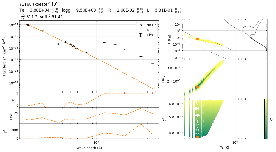
Example 2
import src.binary_sed_fitting as bsf
import warnings
warnings.filterwarnings("ignore")
bsf.console.setLevel(bsf.logging.WARNING)
################################################################################
name        = 'Y1168'
file_name   = 'data/extinction_corrected_flux_files/%s.csv'%name
data        = bsf.load_data(file_name, mode='csv')
distance    = 831. # pc
e_distance  = 11.  # pc

refit    = False
run_name = '0'
################################################################################
model_name = 'koester'
limits = {'Te'   : [5000, 80000],
          'logg' : [ 6.5,   9.5]}
model = bsf.Model(model_name, limits=limits)
################################################################################
star = bsf.Star(name=name,
                distance=distance,
                e_distance=e_distance,
                filters_to_drop=[],
                wavelength_range=[0, 1_000_000_000],
                data=data,
                model=model,
                r_limits='blackbody',
                run_name=run_name)
################################################################################
star.fit_chi2(refit=refit)
star.fit_noisy_chi2(refit=refit)
################################################################################
star.plot(add_noisy_seds=False,
          folder='plots/',
          FR_cutoff=0.5)
star.save_summary()
22:39:56 ----- WARNING  ----- calculate_chi2
Give "refit=True" if you want to rerun the fitting process.
22:39:56 ----- WARNING  ----- get_parameters_from_chi2_minimization
Based on chi2, I recommend removal of following filters: ['WISE/WISE.W1']; chi2=[1722.30668168]
22:39:56 ----- WARNING  ----- calculate_noisy_chi2
Give "refit=True" if you want to rerun the fitting process.
22:39:56 ----- WARNING  ----- get_realistic_errors_from_iterations
logg_A : The best fit value is at upper limit of the model.
Example 3
import src.binary_sed_fitting as bsf
import warnings
warnings.filterwarnings("ignore")
bsf.console.setLevel(bsf.logging.ERROR)
################################################################################
name = 'WOCS2002'
file_name = 'data/extinction_corrected_flux_files/%s.csv'%name
data = bsf.load_data(file_name, mode='csv')
distance = 831. # pc
e_distance = 11. # pc
refit = False
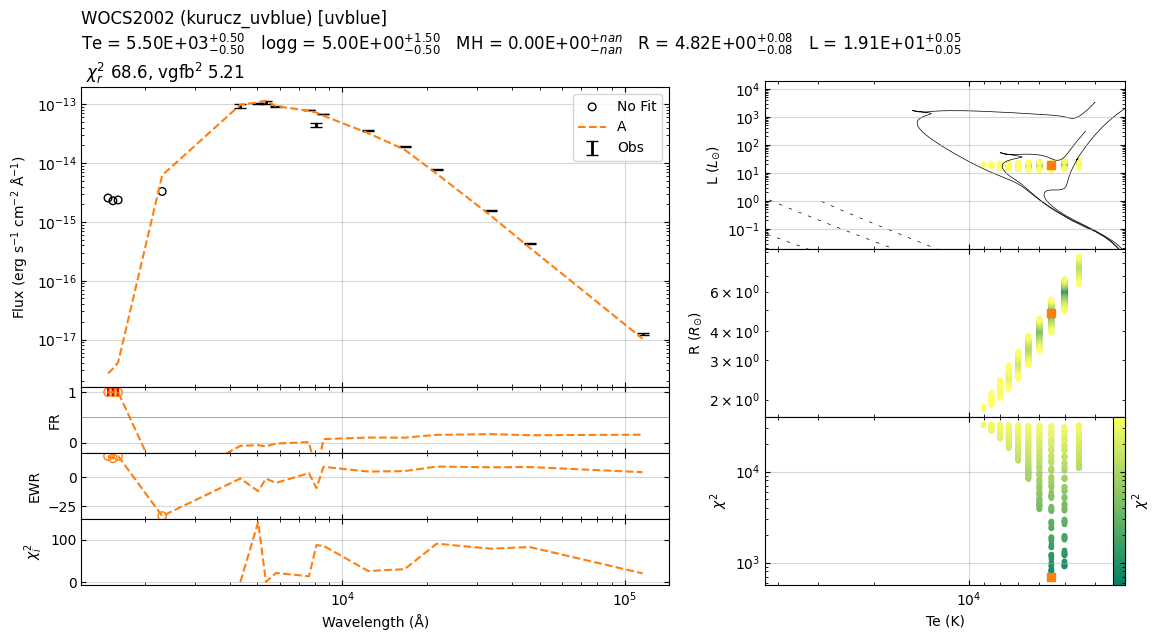
run_name = 'uvblue'
################################################################################
model_name = 'kurucz_uvblue'
limits = {'Te' : [3500, 9000],
'logg' : [ 3, 5],
'MH' : [ 0.0, 0.0]}
model = bsf.Model(model_name, limits=limits)
################################################################################
star = bsf.Star(name=name,
distance=distance,
e_distance=e_distance,
filters_to_drop=[],
wavelength_range=[3000, 1_000_000_000],
data=data,
model=model,
r_limits=[0.1, 10],
run_name=run_name)
################################################################################
star.fit_chi2(refit=refit)
star.fit_noisy_chi2(refit=refit)
################################################################################
star.plot(add_noisy_seds=False,
folder='plots/',
FR_cutoff=0.5)
star.save_summary()
Advance options
Console logging options can be changes based on requirements
For minimal logs:
bsf.console.setLevel(bsf.logging.ERROR)For typical logs:
bsf.console.setLevel(bsf.logging.WARNING)For detailed logs:
bsf.console.setLevel(bsf.logging.INFO)For debug logs:
bsf.console.setLevel(bsf.logging.DEBUG)
Editing the
bsffile and re-importing the filepython import importlib importlib.reload(bsf)Starcomponent: Name of the component. Useful for binary fits.
fit_blackbodyFits a blackbody to given flux
p0: Initial guess for the temperature and log(scaling factor). Default is [5000., -20]
fit_chi2_trim: Trimming the number of chi2 fits to save memory
fit_noisy_chi2total_iterations: Number of iterations for noisy fits
plotshow_plot: Showing/hiding the plots in the notebook
plot_publicDuplicate and modify the funcion to suit your need
create_sf_listLOG_SF_STEPSIZE(=0.01) andLOG_SF_FLEXIBILITY(=2) are used to determine the stepsizes in scaling factor
dataDataframe containing the observational data. It is cropped to the fitted filters based on
filters_to_dropandwavelength_range.
data_allA copy of the original data with an added ‘fitted’ column indicating whether the filter is used. Mmodel flux, residuals, and statistical measures are added in
Fitter.get_parameters_from_chi2_minimizationandFitter.get_parameters_from_noisy_chi2_minimization.
data_not_fittedDataFrame containing only removed filters based on
filters_to_dropandwavelength_range
save_figEdit the function to change the plot format (e.g. PDF, PNG or multiple formats)
Star.df_chi2andStar.df_chi2_noisyThe chi2 dataframes are saved in
outputs\.
log files
The raw log files (with logging level DEBUG) are saved in
data\log_<today's date>.txtThe summary logs are chi2 dataframe is saved in
outputs\log_single_fitting.csvandoutputs\log_starsystem_fitting.csv.
import src.binary_sed_fitting as bsf
import warnings
import importlib
warnings.filterwarnings("ignore")
importlib.reload(bsf)
bsf.console.setLevel(bsf.logging.INFO)
################################################################################
name = 'WOCS2002'
file_name = 'data/extinction_corrected_flux_files/%s.csv'%name
data = bsf.load_data(file_name, mode='csv')
distance = 831. # pc
e_distance = 11. # pc
refit = False
################################################################################
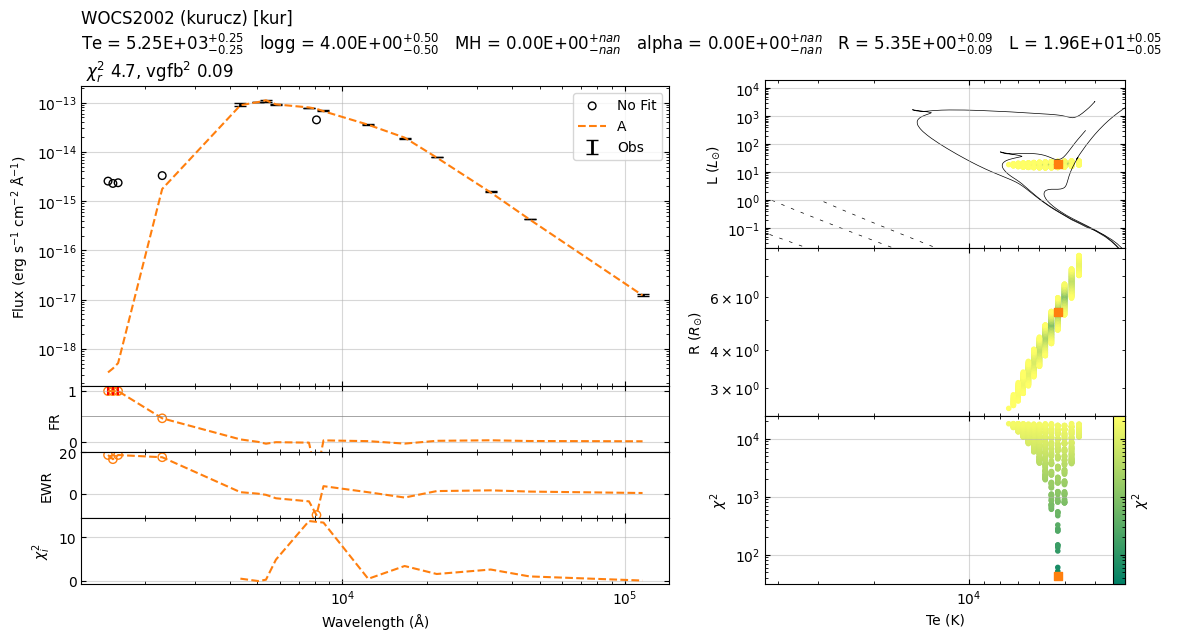
model_name = 'kurucz'
limits = {'Te' : [3500, 9000],
'logg' : [ 3, 5],
'MH' : [ 0.0, 0.0],
'alpha': [ 0.0, 0.0]}
model = bsf.Model(model_name, limits=limits)
################################################################################
star = bsf.Star(name=name,
distance=distance,
e_distance=e_distance,
filters_to_drop=['KPNO/Mosaic.I'],
wavelength_range=[3000, 1_000_000_000],
data=data,
model=model,
r_limits='blackbody',
run_name='kur',
component='A')
################################################################################
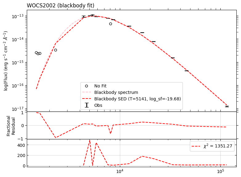
star.fit_blackbody(p0=[5000., -20],
plot=True,
show_plot=True,
folder=None)
################################################################################
star.fit_chi2(refit=refit,
_trim=1000)
star.fit_noisy_chi2(refit=refit,
total_iterations=100)
################################################################################
star.plot(add_noisy_seds=False,
show_plot=True,
folder=None,
FR_cutoff=0.5)
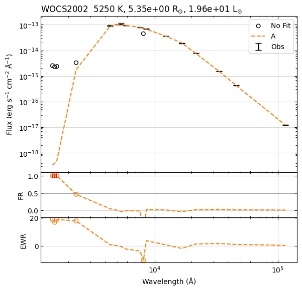
star.plot_public(add_noisy_seds=False,
show_plot=True,
folder=None,
FR_cutoff=0.5)
22:39:59 ----- INFO     ----- __init__
==========================================================
----------------------------------------------------------
------------            WOCS2002 A            ------------
----------------------------------------------------------
==========================================================
22:39:59 ----- INFO     ----- drop_filters
                        Fitted           Not fitted
wavelength
1481.000000                     Astrosat/UVIT.F148W
1541.000000                     Astrosat/UVIT.F154W
1608.000000                     Astrosat/UVIT.F169M
2303.366368                         GALEX/GALEX.NUV
4357.276538      KPNO/Mosaic.B
5035.750275     GAIA/GAIA3.Gbp
5366.240786      KPNO/Mosaic.V
5822.388714       GAIA/GAIA3.G
7619.959993     GAIA/GAIA3.Grp
8101.609574                           KPNO/Mosaic.I
8578.159519    GAIA/GAIA3.Grvs
12350.000000     2MASS/2MASS.J
16620.000000     2MASS/2MASS.H
21590.000000    2MASS/2MASS.Ks
33526.000000      WISE/WISE.W1
46028.000000      WISE/WISE.W2
115608.000000     WISE/WISE.W3
22:39:59 ----- INFO     ----- drop_filters
Filters: used/all = 12/17
22:39:59 ----- INFO     ----- blackbody
Fit parameters: T=5141 K, log_sf=-19.68
22:39:59 ----- INFO     ----- blackbody
Fit parameters: T=5141 K, log_sf=-19.68
22:39:59 ----- WARNING  ----- calculate_chi2
Give "refit=True" if you want to rerun the fitting process.
22:39:59 ----- INFO     ----- calculate_chi2
     Te  logg   MH  alpha            sf       chi2         R          L
0  5250   4.0  0.0    0.0  2.105389e-20  42.148650  5.348053  19.575928
1  5250   4.5  0.0    0.0  2.105389e-20  43.750774  5.348053  19.575928
2  5250   3.5  0.0    0.0  2.105389e-20  46.564792  5.348053  19.575928
3  5250   5.0  0.0    0.0  2.105389e-20  51.654370  5.348053  19.575928
4  5250   3.0  0.0    0.0  2.105389e-20  60.201435  5.348053  19.575928
22:39:59 ----- INFO     ----- get_parameters_from_chi2_minimization
Te  5250
logg        4.0
MH  0.0
alpha       0.0
sf  2.1053889442869984e-20
chi2        42.148649603337915
R   5.348053395835723
L   19.57592810070829
vgf2        11.474651537318044
vgfb2       0.8009328529123378
22:39:59 ----- WARNING  ----- calculate_noisy_chi2
Give "refit=True" if you want to rerun the fitting process.
22:39:59 ----- INFO     ----- calculate_noisy_chi2
     Te  logg   MH  alpha            sf       chi2         R          L
0  5250   4.0  0.0    0.0  2.105389e-20  42.148650  5.348053  19.575928
1  5250   4.0  0.0    0.0  2.105389e-20  48.786377  5.348053  19.575928
2  5250   4.5  0.0    0.0  2.105389e-20  58.784976  5.348053  19.575928
3  5250   4.0  0.0    0.0  2.105389e-20  83.279210  5.348053  19.575928
4  5250   4.0  0.0    0.0  2.105389e-20  57.314788  5.348053  19.575928
22:39:59 ----- INFO     ----- get_parameters_from_noisy_chi2_minimization
Te  5250(-250,+250)
logg        4.0(-0.5,+0.5)
MH  0.0(-nan,+nan)
alpha       0.0(-nan,+nan)
sf  2.1053889442869984e-20(-4.792450334089126e-22,+4.904080842726991e-22)
R   5.348053395835723(-0.09359116353916891,+0.0940563746344943)
L   19.57592810070829(-0.518255617587945,+0.518255617587945)
print(star.data.index)
print(star.data_all.index)
print(star.data_not_fitted.index)
star.data.head()
Index(['KPNO/Mosaic.B', 'GAIA/GAIA3.Gbp', 'KPNO/Mosaic.V', 'GAIA/GAIA3.G',
       'GAIA/GAIA3.Grp', 'GAIA/GAIA3.Grvs', '2MASS/2MASS.J', '2MASS/2MASS.H',
       '2MASS/2MASS.Ks', 'WISE/WISE.W1', 'WISE/WISE.W2', 'WISE/WISE.W3'],
      dtype='object', name='FilterID')
Index(['Astrosat/UVIT.F148W', 'Astrosat/UVIT.F154W', 'Astrosat/UVIT.F169M',
       'GALEX/GALEX.NUV', 'KPNO/Mosaic.B', 'GAIA/GAIA3.Gbp', 'KPNO/Mosaic.V',
       'GAIA/GAIA3.G', 'GAIA/GAIA3.Grp', 'KPNO/Mosaic.I', 'GAIA/GAIA3.Grvs',
       '2MASS/2MASS.J', '2MASS/2MASS.H', '2MASS/2MASS.Ks', 'WISE/WISE.W1',
       'WISE/WISE.W2', 'WISE/WISE.W3'],
      dtype='object', name='FilterID')
Index(['Astrosat/UVIT.F148W', 'Astrosat/UVIT.F154W', 'Astrosat/UVIT.F169M',
       'GALEX/GALEX.NUV', 'KPNO/Mosaic.I'],
      dtype='object', name='FilterID')
| wavelength | flux | error | error_fraction | error_2percent | error_10percent | log_wavelength | log_flux | e_log_flux | fitted | ... | chi2_i | vgf2_i | vgfb2_i | model_flux_median | residual_flux_median | fractional_residual_median | ewr_median | chi2_i_median | vgf2_i_median | vgfb2_i_median | |
|---|---|---|---|---|---|---|---|---|---|---|---|---|---|---|---|---|---|---|---|---|---|
| FilterID | |||||||||||||||||||||
| KPNO/Mosaic.B | 4357.276538 | 9.309407e-14 | 6.130611e-15 | 0.065854 | 6.130611e-15 | 9.309407e-15 | 3.639215 | -13.031078 | 0.028600 | 1 | ... | 0.545712 | 0.545712 | 2.366611e-01 | 8.856525e-14 | 4.528824e-15 | 0.048648 | 0.738723 | 0.545712 | 0.545712 | 2.366611e-01 |
| GAIA/GAIA3.Gbp | 5035.750275 | 1.028575e-13 | 3.881303e-16 | 0.003773 | 2.057150e-15 | 1.028575e-14 | 3.702064 | -12.987764 | 0.001639 | 1 | ... | 0.000081 | 0.000003 | 1.148069e-07 | 1.028540e-13 | 3.485137e-18 | 0.000034 | 0.008979 | 0.000081 | 0.000003 | 1.148069e-07 |
| KPNO/Mosaic.V | 5366.240786 | 1.079375e-13 | 7.108112e-15 | 0.065854 | 7.108112e-15 | 1.079375e-14 | 3.729670 | -12.966827 | 0.028600 | 1 | ... | 0.298089 | 0.298089 | 1.292734e-01 | 1.118184e-13 | -3.880853e-15 | -0.035955 | -0.545975 | 0.298089 | 0.298089 | 1.292734e-01 |
| GAIA/GAIA3.G | 5822.388714 | 9.174216e-14 | 2.539155e-16 | 0.002768 | 1.834843e-15 | 9.174216e-15 | 3.765101 | -13.037431 | 0.001202 | 1 | ... | 4.897209 | 0.093784 | 3.751362e-03 | 9.230407e-14 | -5.619057e-16 | -0.006125 | -2.212964 | 4.897209 | 0.093784 | 3.751362e-03 |
| GAIA/GAIA3.Grp | 7619.959993 | 7.878734e-14 | 3.154436e-16 | 0.004004 | 1.575747e-15 | 7.878734e-15 | 3.881953 | -13.103544 | 0.001739 | 1 | ... | 13.712759 | 0.549535 | 2.198141e-02 | 7.995545e-14 | -1.168111e-15 | -0.014826 | -3.703074 | 13.712759 | 0.549535 | 2.198141e-02 |
5 rows × 24 columns